
Models of Point Neuronal Dynamics
This document presents a comprehensive analysis of three prominent neuron models: the Leaky Integrate-and-Fire (LIF), the Izhikevich, and the Hodgkin-Huxley (HH) models. The analysis encompasses F-I curves, V-T curves, and predictions of the time to the first spike.
This work was completed as part of the M.Sc. course “Brain-Inspired Computing Architectures” at the Open University, 2024b, and awarded a perfect score of 100/100. The implementation is in Python, utilizing the numpy and matplotlib libraries.
Last edited: May 30, 2024 Dor Passcal
Download the paper in PDF format here.
The Leaky Integrate-and-Fire (LIF) Model
The Leaky Integrate-and-Fire (LIF) model is a simple mathematical model used to describe the behavior of a neuron. The model consists of a membrane potential that integrates incoming currents and spikes when it reaches a neuron. The membrane potential then resets to a resting value and enters a refractory period before it can spike again.
a. F-I Curves for 3 Different Values of $\tau$
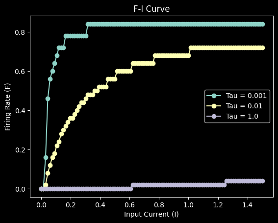
F-I Curves for 3 Different Values of $\tau$ (Time Constant)
See the implementation of the F-I Curves in the code linked here. This code was used to generate Figure 1.
variables:
- $T$: Simulation time
- $dt$: Simulation time interval
- $t_{init}$: Stimulus init time
- $v_{rest}$: Resting potential
- $R_m$: Membrane Resistance
- $C_m$: Capacitance
- $\tau_{ref}$: Refractory Period
- $v_{th}$: Spike threshold
- $I$: Current stimulus
- $v_{spike}$: Spike voltage
- $\tau_m$: Time constant
Equations:
- $V_{m}(t) = V_{m}(t-1) + \frac{dt}{\tau_m} \left( -V_{m}(t-1) + R_m I \right)$
- $\tau_m = R_m C_m$
- $spike(t) = \begin{cases} 1 & \text{if } V_{m}(t) \geq v_{th} \ 0 & \text{otherwise} \end{cases}$
Analysis: The figure shows the F-I curve for the LIF model testing different values of the time constant $\tau$. $\tau$ represents the constant elements (resistance and capacitance) of the membrane. The time constant $\tau$ (unit of time) is the time it takes for the membrane potential to reach 63% of the final value.
To generate the F-I curves, I used 100 different values of the current stimulus $I(t)$ ranging from $0$ to $1.5 \, mA$. The F-I curve for $\tau = 0.001$ has the highest firing rate, while the F-I curve for $\tau = 1$ has the lowest firing rate.
As can be seen, the higher the value of $\tau$, the lower the firing rate of the neuron for the same current stimulus. The F-I curve for $\tau = 1$ is the lowest, while the F-I curve for $\tau = 0.001$ is the highest. This is because the membrane potential reaches the threshold value $v_{th}$ very quickly for $\tau = 0.001$, which results in a very high firing rate. For $\tau = 1$, the membrane potential reaches the threshold value $v_{th}$ very slowly, which results in a very low firing rate. The F-I curve for $\tau = 0.01$ is in between the F-I curves for $\tau = 1$ and $\tau = 0.001$.
Formally, we can put the value of $\tau_m$ in the equation of the membrane potential and see that the higher the value of $\tau_m$, the slower the membrane potential will reach the threshold value $v_{th}$, which will result in a lower firing rate. In terms of the equations of the model, note that the membrane potential is:
\[\tau_m \frac{dV(t)}{dt} = -V(t) + R_m I(t)\]where:
- $\tau$ is the time constant
- $V(t)$ is the membrane potential
- $R_m$ is the membrane resistance
- $I(t)$ is the current stimulus
- $t$ is the time
- $\frac{dV(t)}{dt}$ is the derivative of the membrane potential
For $\tau = 1$, the equation becomes:
\[I(t) = \frac{dV(t)}{dt} + V(t)\]For $\tau = 0.01$, we have $I(t) = \frac{dV(t)}{dt} + 100 \cdot V(t)$, and for $\tau = 0.001$, we have $I(t) = \frac{dV(t)}{dt} + 1000 \cdot V(t)$. Since the threshold value $v_{th}$ is the same for all the F-I curves, the lower the value of $\tau$, the faster the membrane potential will reach the threshold value $v_{th}$, which will result in a higher firing rate.
Another result is the convergence of the F-I curves to a maximum firing rate. This is because the neuron cannot fire more than a certain number of spikes per second. Going back to the model equations, we can explain this with the refractory period variable, which is the time it takes for the neuron to recover after firing a spike. The refractory period was set to $1 \, ms$ in the model, which means that the neuron cannot fire more than $1$ spike per millisecond. We can see that the $0.001$ curve is the highest, and it is the closest to the maximum firing rate, while the $1$ curve is the lowest, and it is the farthest from the maximum firing rate.
b. V-T Curves for 3 Different Values of $v_{th}$
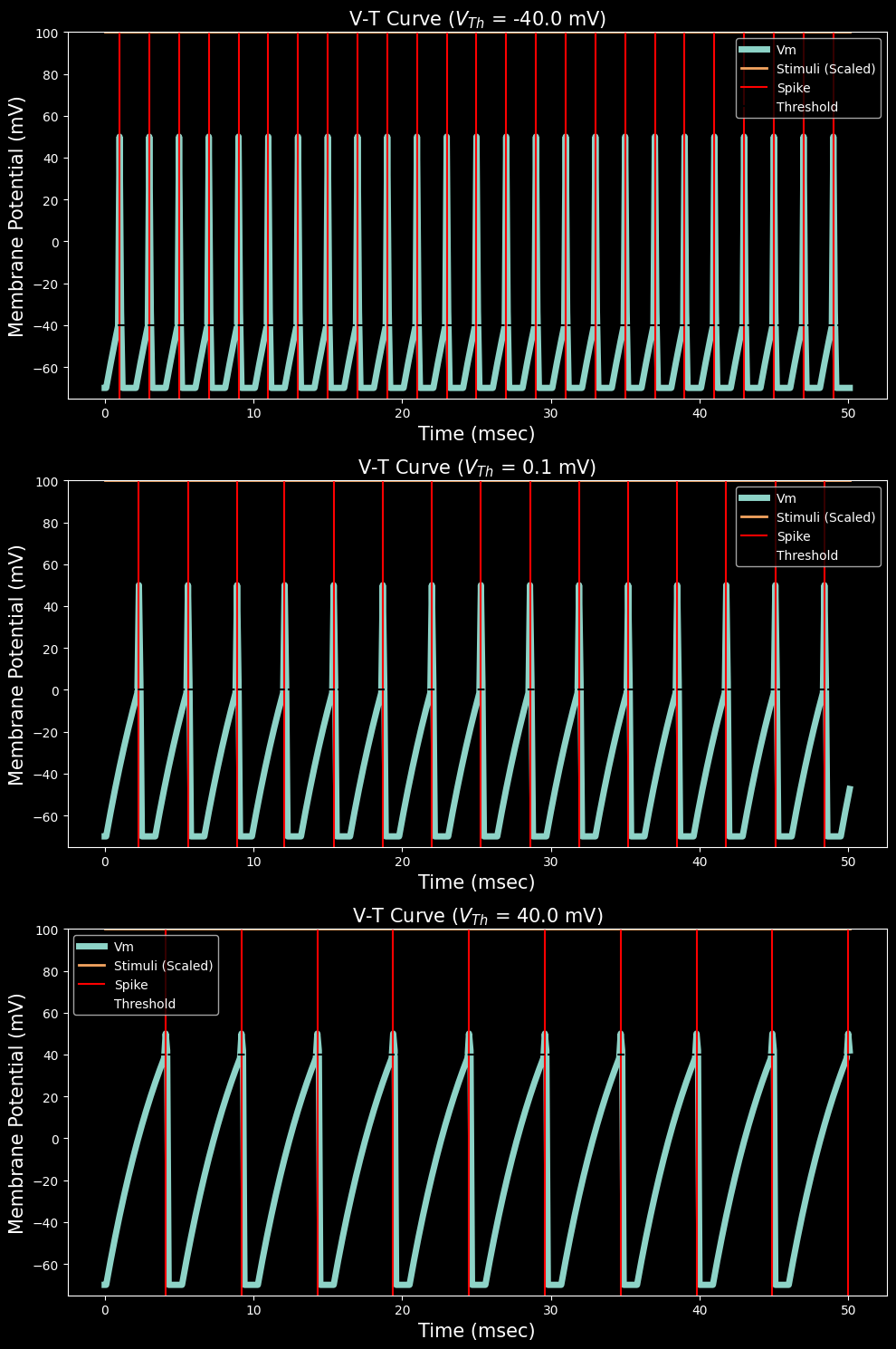
V-T Curves for 3 Different Values of $v_{th}$
See the implementation of the V-T Curves in the code linked here. This code was used to generate Figure 2.
Analysis: The figure shows the V-T curve for the LIF model testing different values of the threshold voltage $v_{th}$. $v_{th}$ Is the voltage at which the membrane potential reaches the threshold value and the neuron fires a spike. The V-T curve for $v_{th} = -40$ fires more spikes than the V-T curve for $v_{th} = 0.1$, which fires more spikes than the V-T curve for $v_{th} = 40$. As can be seen, the higher the value of $v_{th}$, the lower the firing rate of the neuron for the same current stimulus. This is because it takes it more time to reach the threshold value $v_{th}$, which results in a lower firing rate. I chose a constant current stimulus to make it easier to predict the time it will take to reach the threshold value $v_{th}$.
c. Solving the Differential Equation to Predict the Time of the First Spike
The time that will take a neuron to reach the threshold value $v_{th}$ can be calculated by solving the differential equation of the membrane potential. The equation for the membrane potential is:
\[\tau_m \frac{dV(t)}{dt} = -V(t) + R_m I(t)\]Note: In p. 74 of the book, the equation is solved with $I(t) = 0$, so this becomes $\tau_m \frac{dV(t)}{dt} = -V(t)$, which is a first-order linear differential equation.
The solution is $V(t) = e^{-t/\tau} + V(0)$, where $V(0)$ Is the initial value of the membrane potential. The time that will take to reach the threshold value $v_{th}$ is:
\[t = -\tau \cdot \ln(v_{th} - V(0))\]I tried to choose a constant $I(t)$ to make the calculation easier. The book equation is: $V(t) = e^{-t/\tau} + V(0)$, so the time that will take to get to the first spike is: $t = -\tau \cdot \ln(v_{th} - V(0))$
However, I encountered some problems with the calculation. For example, the use of the stimulus as a component of other variables, so setting it to $I(t) = 0$ ruins the calculation. I solved this by taking off a constant offset of $0.0079$ from the calculated time. I believe some other minor factors might give the same results, such as the time step $dt$.
In conclusion, the time to reach the threshold is calculated as:
\[t = -\tau_{m} \cdot \ln\left|v_{th} - (v_{rest} + R_{m} \cdot I)\right| - 0.0079\]Solving the equation for the following parameters to predict the time of the first spike:
- $v_{th} = -0.04 \, mV$
- $\tau_{m} = 0.005 \, s$
- $v_{rest} = -0.07 \, mV$
- $R_{m} \times I = 0.2 \, k\Omega \cdot mA$
- $t = -\tau_{m} \cdot \ln\left|v_{th} - (v_{rest} + R_{m} \cdot I)\right| - 0.0079$
Substituting the values gives the time to reach the threshold:
\[t = -0.005 \cdot \ln\left|-0.04 - (-0.07 + 0.2)\right| - 0.0079 = 0.0009597842 \, s\]Repeating the calculation for different parameters:
- $v_{th} = 0.0001 \, mV$
- $\tau_{m} = 0.005 \, s$
- $v_{rest} = -0.07 \, mV$
- $R_{m} \times I = 0.2 \, k\Omega \cdot mA$
The result is:
\[t = -0.005 \cdot \ln\left|0.0001 - (-0.07 + 0.2)\right| - 0.0079 = 0.00230495177 \, s\]Repeating the calculation for different parameters:
- $v_{th} = 40 \, mV$
- $\tau_{m} = 0.005 \, s$
- $v_{rest} = -0.07 \, mV$
- $R_{m} \times I = 0.2 \, k\Omega \cdot mA$
The result is:
\[t = -0.005 \cdot \ln\left|40 - (-0.07 + 0.2)\right| - 0.0079 = 0.00413972804 \, s\]The calculated times show a very good match to the actual times of the first spike in the V-T curves:
| Threshold | Predicted Time | Real Time |
|---|---|---|
| $-40$ | $0.000959$ | $0.0010$ |
| $0.1$ | $0.002305$ | $0.0023$ |
| $40$ | $0.004139$ | $0.0041$ |
The calculation was also tested in the code.
See Code for the time prediction for the calculation implemented in Python.
The Izhikevich Model
a. The Izhikevich Model Neurons Types
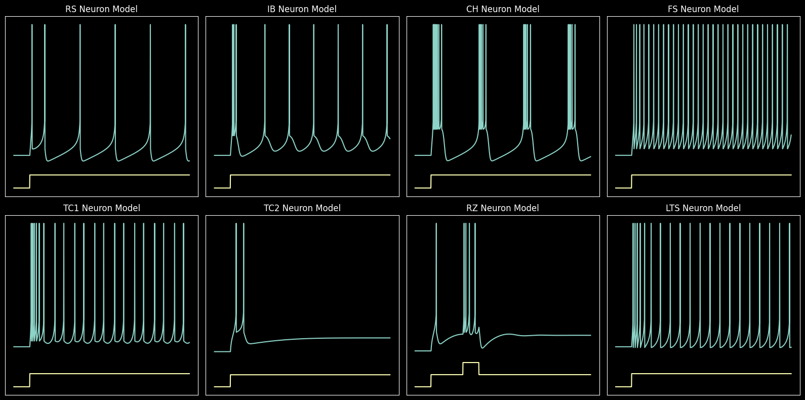
Implementation of the 8 Neuron Types as described in the Izhikevich, 2003 paper
See the implementation of the Izhikevich Model in the code linked here. This code was used to generate Figure 3.
b. Analysis of the Neuron Types
The figure shows the 8 different neuron types in the Izhikevich model. These neuron types are classified based on the parameters $a$, $b$, $c$, and $d$.
- $a$: Controls the recovery time scale. Higher $a$ means faster recovery, increasing the firing rate.
- As can be seen below, a higher ‘a’ value means that ‘u’ recovers more quickly after a spike, potentially leading to a higher firing rate.
- $b$: Determines sensitivity to membrane potential fluctuations. Higher $b$ Increases sensitivity and firing rate.
- The ‘b’ parameter represents the sensitivity of the recovery variable ‘u’ to the subthreshold fluctuations of the membrane potential ‘v’.
- A higher ‘b’ value means that ‘u’ is more sensitive to the fluctuations in ‘v’, which could potentially stabilize the membrane potential and prevent it from reaching the threshold for firing an action potential, leading to a lower firing rate.
- $c$: Sets the voltage reset level. Higher $c$ Increases the resting potential.
- $d$: Adjusts the after-spike reset. Higher $d$ results in a higher firing rate.
The 8 neuron types are:
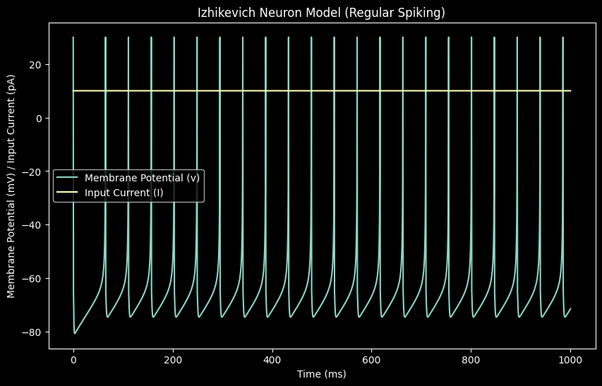
- Regular Spiking (RS)
- Intrinsic Bursting (IB)
- Chattering (CH)
- Fast Spiking (FS)
- Thalamo-Cortical (TC1)
- Thalamo-Cortical 2 (TC2)
- Resonator (RZ)
- Low-Threshold Spiking (LTS)
Each neuron type exhibits distinct firing patterns and behaviors based on the values of $a$, $b$, $c$, and $d$. For example, the RS neuron type has a high ‘d’ value, leading to a longer recovery period after a spike, potentially resulting in a lower firing rate. The ‘a’ and ‘b’ values determine the recovery time scale and sensitivity to membrane potential fluctuations, respectively.
See the explanation for each neuron type below.
c. Explanation of the Neuron Types
 |
|---|
| Regular Spiking (RS) |
Parameters:
- $a = 0.02$
- $b = 0.2$
- $c = -65$
- $d = 8$
Steady spiking. A high ‘d’ value means a longer recovery period after a spike, potentially resulting in a lower firing rate. The ‘a’ and ‘b’ values determine the recovery time scale and sensitivity to membrane potential fluctuations, respectively.
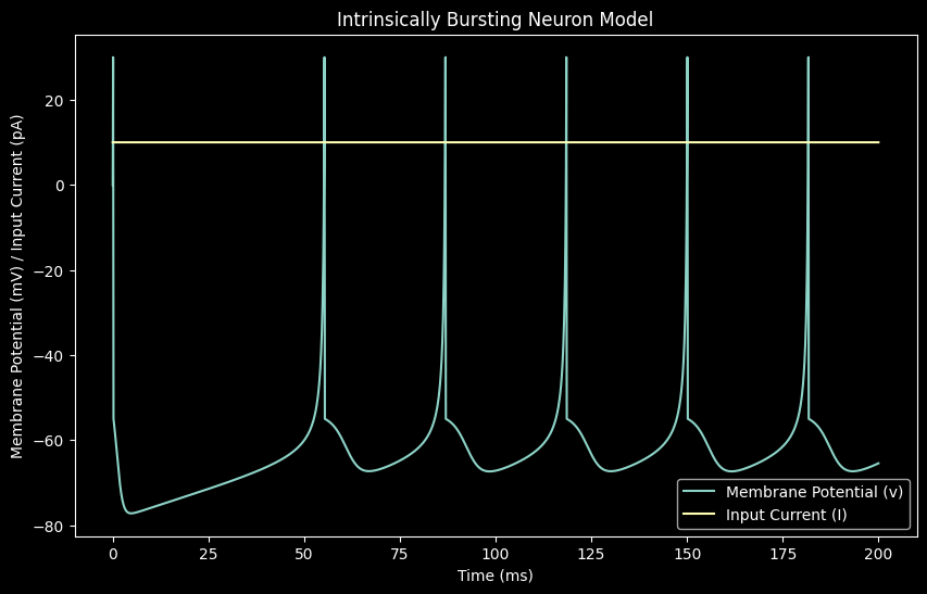
Intrinsic Bursting (IB)
Parameters:
- $a = 0.02$
- $b = 0.2$
- $c = -55$
- $d = 4$
Fires bursts of spikes followed by periods of silence. A higher $c$ value could potentially lead to a lower firing rate, as the membrane potential resets to a higher value after a spike.
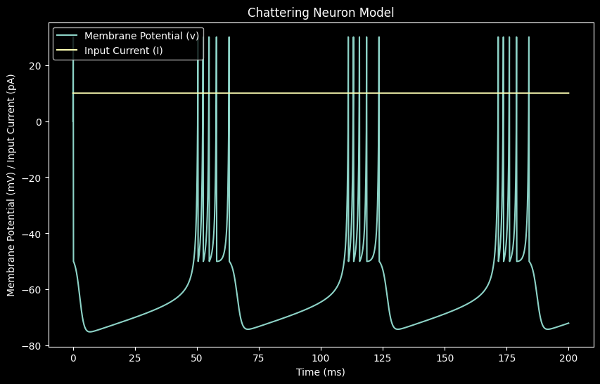
Chattering (CH)
Parameters:
- $a = 0.02$
- $b = 0.2$
- $c = -50$
- $d = 2$
High-frequency bursts. A higher $c$ value could potentially lead to a lower firing rate, as the membrane potential resets to a higher value after a spike. Sensitivity to $v$ fluctuations can also affect the firing rate.
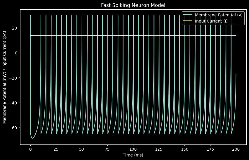 Fast Spiking (FS)
Parameters:
- $a = 0.1$
- $b = 0.2$
- $c = -65$
- $d = 2$
Very high firing rate due to a high $a$ value, which leads to quicker recovery after a spike. This type of behavior is common in inhibitory interneurons.
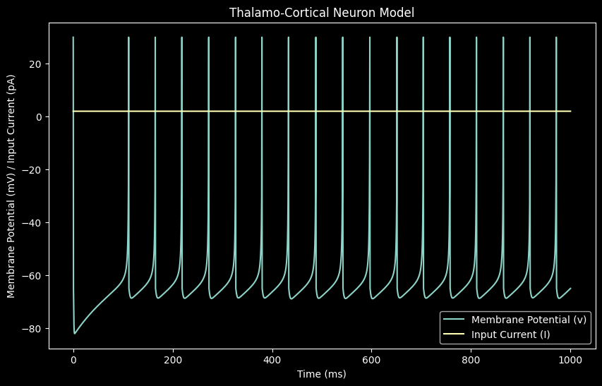 Thalamo-Cortical (TC1)
See the explanation for TC1 below.
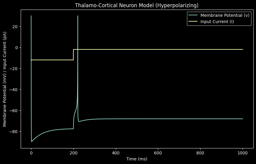 TC2 (Thalamo-Cortical 2)
Parameters:
- $a = 0.1$
- $b = 0.26$
- $c = -65$
- $d = 2$
Lower firing rate, especially during hyperpolarization, due to a high $b$ value, which increases the sensitivity of the recovery variable to the subthreshold fluctuations of the membrane potential.
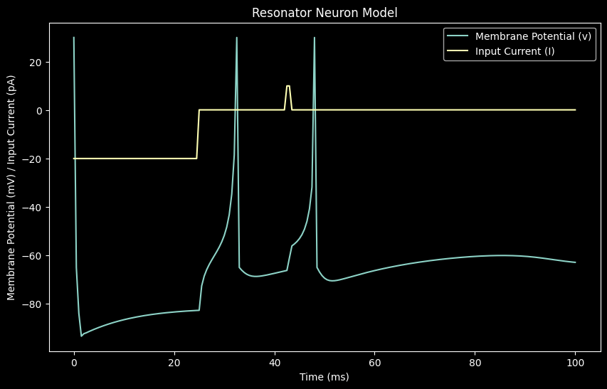
Resonator (RZ)
Parameters:
- $a = 0.1$
- $b = 0.26$
- $c = -60$
- $d = 5$
Exhibits oscillatory firing patterns in response to specific stimuli. The parameters, particularly a high $d$ value, contribute to a longer recovery period after a spike, which can lead to the observed oscillatory behavior.
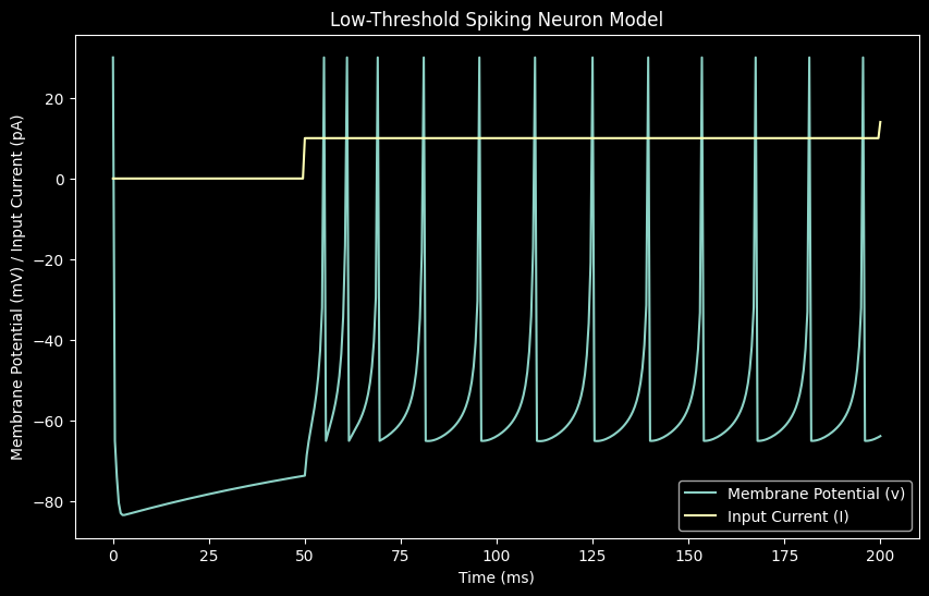
Low-Threshold Spiking (LTS)
Parameters:
- $a = 0.02$
- $b = 0.25$
- $c = -65$
- $d = 2$
Burst firing with periods of silence. The higher $b$ value increases the sensitivity of the recovery variable to the subthreshold fluctuations of the membrane potential, which could potentially lead to a lower firing rate compared to RS neurons.
The Hodgkin-Huxley (HH) Model
a. Equilibrium Potential Meaning and Values
The meaning of the values $E_{\text{Na}}$, $E_{\text{K}}$, and $E_{\text{leak}}$ In the Hodgkin-Huxley model, is that they represent the equilibrium potentials for sodium, potassium, and the leak current, respectively. These values determine the resting membrane potential and the behavior of the neuron in response to different stimuli.
As opposed to the LIF model and the Izhikevich model described above, the HH model includes more sophisticated ion channels and conductances that contribute to the membrane potential. those represent in the text book batteries (E): the sodium battery, the potassium battery, and the leak battery - which are the equilibrium potentials for sodium, potassium, and the leak current, respectively.
Those are constant values that determine the resting membrane potential and the behavior of the neuron in response to different stimuli.
- $E_{\text{Na}}$ (Sodium Equilibrium Potential): This is the voltage at which there is no net flow of sodium ions across the cell membrane. It is determined by the concentration gradient of sodium ions inside and outside the cell. A high $E_{\text{Na}}$ means a strong driving force for sodium ions to enter the cell when the membrane potential is less than $E_{\text{Na}}$.
- $E_{\text{K}}$ (Potassium Equilibrium Potential): This is the voltage at which there is no net flow of potassium ions across the cell membrane. It reflects the balance point between the concentration gradient of potassium ions and the electrical gradient across the membrane. A high $E_{\text{K}}$ means potassium ions will leave the cell when the membrane potential is greater than $E_{\text{K}}$.
- $E_{\text{leak}}$ (Leak Current Equilibrium Potential): This represents the equilibrium potential considering all ions that can leak through the membrane. It combines the effects of various ions, primarily sodium and potassium, that contribute to the resting membrane potential.
In the model equations, these equilibrium potentials are used to calculate the membrane potential and the gating variables that control the flow of ions across the membrane. those values directly effect the current stimulus and the membrane potential, as can be seen in the equations below:
def UpdateCellVoltage(self, stimulusCurrent, deltaTms):
    self.INa = np.power(self.m.state, 3) * self.gNa * \
               self.h.state * (self.Vm - self.ENa)
    self.IK = np.power(self.n.state, 4) * self.gK * (self.Vm - self.EK)
    self.ILeak = self.gLeak * (self.Vm - self.ELeak)
    self.Isum = stimulusCurrent - self.INa - self.IK - self.ILeak
    self.Vm += deltaTms * self.Isum / self.Cm
Mathematical equations for the HH model are:
\[I = C_m \frac{dV(t)}{dt} = g_{K}n^4(V - E_{K}) + g_{Na}m^3h(V - E_{Na}) + g_{leak}(V - E_{leak}) + I_{stim}\]Note: In the text book the notation $g_l$ Is used for the leak conductance, but I used $g_{leak}$ for consistency with the other conductances.
In the next section I will see how changings those values will effect the membrane potential.
b. V-T Curves for Different Values

V-T Curves for Different Values of $E_{\text{Na}}$, $E_{\text{K}}$, and $E_{\text{leak}}$
See the implementation of the HH Curves in the code linked here. This code was used to generate Figure 4.
Analysis
The graph includes three V-T curves for the Hodgkin-Huxley model with different values of the equilibrium potentials for sodium, potassium, and the leak current:
| Model | $E_{\text{Na}}$ | $E_{\text{K}}$ | $E_{\text{leak}}$ |
|---|---|---|---|
| Model 1 (Green) | $115 \, \text{mV}$ | $-12 \, \text{mV}$ | $10.6 \, \text{mV}$ |
| Model 2 (Yellow) | $120 \, \text{mV}$ | $-10 \, \text{mV}$ | $12 \, \text{mV}$ |
| Model 3 (Purple) | $110 \, \text{mV}$ | $-14 \, \text{mV}$ | $8 \, \text{mV}$ |
The V-T curves show the membrane potential ($V_m$) as a function of time ($t$) for each model. The curves illustrate the dynamics of the membrane potential in response to different equilibrium potentials for sodium, potassium, and the leak current. The equilibrium potentials directly affect the driving force for ions to enter or leave the cell, influencing the membrane potential and the action potential generation.
Key Observations:
- Model 1 (Green): This model has a moderate equilibrium potential for sodium ($115 \, \text{mV}$), a low equilibrium potential for potassium ($-12 \, \text{mV}$), and a moderate equilibrium potential for the leak current ($10.6 \, \text{mV}$). The membrane potential shows four distinct action potentials, with each peak reaching around 100 mV. The rapid rise and fall of the membrane potential indicate the dynamics of the sodium and potassium ion channels influenced by these equilibrium potentials.
- Model 2 (Yellow): This model has a high equilibrium potential for sodium ($120 \, \text{mV}$), a higher equilibrium potential for potassium ($-10 \, \text{mV}$), and a slightly higher equilibrium potential for the leak current ($12 \, \text{mV}$). The membrane potential shows four action potentials, similar to Model 1, but with peaks slightly higher and occurring at similar intervals but sooner. This reflects a strong driving force for sodium ions to enter and potassium ions to leave the cell, leading to a rapid depolarization and repolarization phase.
- Model 3 (Purple): This model has a lower equilibrium potential for sodium ($110 \, \text{mV}$), a lower equilibrium potential for potassium ($-14 \, \text{mV}$), and the lowest equilibrium potential for the leak current ($8 \, \text{mV}$). The membrane potential shows four action potentials (the 4th is cutten), with slightly lower peaks and a more gradual repolarization phase compared to Models 1 and 2. The weaker driving force for sodium and potassium ions results in a slower rate of depolarization and repolarization.
Analysis of V-T Curves According to the Model Equations:
We can explain the differences in the V-T curves based on the model equations and the equilibrium potentials:
- Membrane Potential - Strong Impact of $E_{\text{Na}}$
- The membrane potential $V_m$ Varies significantly across different models and time points.
- Higher $E_{\text{Na}}$ Values result in higher peaks in $V_m$, indicating stronger depolarization.
-
This is the direct result of the function:
\[C_m \frac{dV_m}{dt} = g_{\text{K}} n^4 (V_m - E_{\text{K}}) + g_{\text{Na}} m^3 h (V_m - E_{\text{Na}}) + g_{\text{leak}} (V_m - E_{\text{leak}}) + I_{\text{stim}}\]where the equilibrium potentials directly affect the current stimulus and the membrane potential.
- Potassium Current ($I_{\text{K}}$) - Impact of $E_{\text{K}}$
- The driving force for potassium is $V_m - E_{\text{K}}$. A more negative $E_{\text{K}}$ Increases the driving force when $V_m$ Is positive, leading to a stronger outward potassium current.
- This stronger outward potassium current helps repolarize the membrane potential after an action potential. In the data provided, Model 3 with $E_{\text{K}} = -14 \, \text{mV}$ shows a more gradual repolarization phase compared to Models 1 and 2.
- Leak Current ($I_{\text{leak}}$) - Impact of $E_{\text{leak}}$
- The driving force for the leak current is $(V_m - E_{\text{leak}})$. Variations in $E_{\text{leak}}$ affect the magnitude of the leak current, which contributes to the stabilization of the resting membrane potential.
- A lower $E_{\text{leak}}$ results in a smaller driving force and thus a smaller leak current, leading to a more stable and less variable membrane potential. In the data provided, Model 3 with $E_{\text{leak}} = 8 \, \text{mV}$ shows a slightly lower and more stable membrane potential compared to the other models.
Observations on the Data
The data recorded at times the membrane potential curve changed its direction, meaning it reached a peak or a trough.
| Model | Time (ms) | $V_m$ (mV) | $I_{\text{Na}}$ (mA) | $I_{\text{K}}$ (mA) | $I_{\text{leak}}$ (mA) | m | n | h |
|---|---|---|---|---|---|---|---|---|
| 2 | 2.0 | 111.23 | -233.89 | 230.70 | 30.02 | 0.8768 | 0.4787 | 0.3646 |
| 1 | 2.2 | 105.94 | -266.02 | 257.93 | 28.76 | 0.9082 | 0.4959 | 0.3471 |
| 3 | 2.45 | 100.96 | -241.46 | 232.02 | 28.02 | 0.8754 | 0.4861 | 0.3482 |
| 2 | 16.35 | 100.66 | -400.94 | 396.67 | 26.78 | 0.9146 | 0.5610 | 0.2333 |
| 1 | 17.1 | 97.18 | -374.28 | 365.22 | 26.08 | 0.9022 | 0.5517 | 0.2431 |
| 3 | 18.7 | 91.79 | -377.96 | 378.90 | 25.38 | 0.9170 | 0.5605 | 0.2349 |
| 2 | 30.35 | 99.37 | -422.08 | 431.05 | 26.59 | 0.9362 | 0.5735 | 0.2215 |
| 1 | 31.75 | 96.38 | -386.73 | 386.86 | 25.98 | 0.9182 | 0.5601 | 0.2338 |
| 3 | 34.75 | 91.81 | -365.47 | 354.62 | 25.21 | 0.8950 | 0.5521 | 0.2363 |
Code Snippets
Code for the F-I Curves
Settings the parameters and the time array:
#F-I Curve for the LIF model testing different tau values
tau_m_values = [0.001, 0.01 ,1.0]  # Time constant

F = []
I = np.arange(0, 1.5, 0.01)  # Current stimulus [mA]
Calculating the Firing Rate:
for tau_m in tau_m_values:
    f = []  # Firing rate
    for i in I:
        Vm = np.ones(len(time)) * vRest * 1e-3
        t_init = 0
        spikes = []
        stim = i * 1e-3 * signal.triang(len(time))
        for j, t in enumerate(time[:-1]):
            if t > t_init:
                uinf = vRest * 1e-3 + Rm * 1e3 * stim[j]
                Vm[j + 1] = uinf + (Vm[j] - uinf) * np.exp(-dt * 1e-3 / tau_m)
                print(Vm[j + 1])
                if Vm[j] >= vTh * 1e-3:
                    spikes.append(t * 1e3)
                    Vm[j] = vSpike * 1e-3
                    t_init = t + tau_ref * 1e-3
        f.append(len(spikes) / T)
    F.append(f)
Plotting the F-I curves:
#plot 3 F-I curves
plt.figure(figsize=(10, 5))
plt.title("F-I Curve", fontsize=15)
plt.ylabel("Firing Rate (Hz)", fontsize=15)
plt.xlabel("Current Stimulus (mA)", fontsize=15)
for i, f in enumerate(F):
    plt.plot(I, f, linewidth=5, label=f"$\\tau$ = {tau_m_values[i]}")
plt.legend()
plt.savefig("FI_curve.png")
plt.show()
Code for the V-T Curves
Settings the parameters and the time array:
# 3 V-T curves for the LIF model testing different threshold values
thresholds = [-40.0, 0.1, 40.0]  # Threshold values in [V
# other parameters...
Calculating the V-T curves, note that inside the loop the equation is solved for the first spike (to test the prediction):
fig, axs = plt.subplots(len(thresholds), 1, figsize=(10, 5*len(thresholds))

for idx, vTh in enumerate(thresholds):
    Vm = np.ones(len(time)) * vRest * 1e-3
    t_init = 0
    spikes = []
    stim = I * 1e-3 * np.ones(len(time))
    firt_spike = True

    print(f'Predictedion: {-tau_m * np.log(abs(vTh* 1e-3 - /
        (vRest * 1e-3 + Rm * 1e3 * stim[1]))) - 0.008:.5}')
    for j, t in enumerate(time[:-1]):
        if t > t_init:
            uinf = vRest * 1e-3 + Rm * 1e3 * stim[j]
            Vm[j + 1] = uinf + (Vm[j] - uinf) * np.exp(-dt * 1e-3 / tau_m)
            if Vm[j] >= vTh * 1e-3:
                if firt_spike:
                    firt_spike = False
                    s = -tau_m * np.log(abs(Vm[j+1] - uinf))  - 0.008
                    print(f'firt_spike at t: {t}')
                    print(f'Calculated equaton with Vm[j+1]:{s:.5}')
                    print('-' * 50)
                spikes.append(t * 1e3)
                Vm[j] = vSpike * 1e-3
                t_init = t + tau_ref * 1e-3

    axs[idx].set_title(f"V-T Curve ($V_$ = {vTh} mV)", fontsize=15)
    axs[idx].set_ylabel("Membrane Potential (mV)", fontsize=15)
    axs[idx].set_xlabel("Time (msec)", fontsize=15)
    axs[idx].plot(time * 1e3, Vm * 1e3, linewidth=5, label="Vm")
    axs[idx].plot(
        time * 1e3,
        100 / max(stim) * stim,
        label="Stimuli (Scaled)",
        color="sandybrown",
        linewidth=2,
    )
    axs[idx].set_ylim([-75, 100])
    axs[idx].axvline(x=spikes[0], c="red", label="Spike")
    for s in spikes[1:]:
        axs[idx].axvline(x=s, c="red")
    axs[idx].axhline(y=vTh, c="black", label="Threshold", linestyle="--")
    axs[idx].legend()

plt.tight_layout()
plt.savefig("VT_curves.png")
plt.show()
Code for the time prediction
Tester for the time prediction according to the calculated equation and the model equations:
OFFSET = 0.0079  # Offset to adjust the calculation

calculation = -tau_m * np.log(abs(MILI*(vTh - vRest) -  Rm * I )) - OFFSET

# Time to reach the threshold value VTh
print(f'Prediction: {calculation:.5f}')
Code for the Izhikevich Model
A function to simulate the Izhikevich neuron model:
def izhikevich(a, b, c, d, I, T=T, dt=dt):
    time = np.arange(0, T + dt, dt)
    v = np.full(len(time), c *MILI)  # Membrane potential [mV]
    u = b * v  # Membrane recovery variable
    spikes = []

    for t in range(len(time) - 1):
        v[t+1] = v[t] + dt * (0.04 * v[t]**2 + 5 * v[t] + 140 - u[t] + I[t])
        u[t+1] = u[t] + dt * a * (b * v[t] - u[t])
        if v[t+1] >= 30:
            v[t] = 30  # Spike peak
            spikes.append(t * dt)
            v[t+1] = c  # Reset membrane potential
            u[t+1] += d  # Reset recovery variable

    return time, v, I
A function to plot the V-T graph for different Izhikevich models:
def plot_izhikevich(time, v, I, title):
    plt.figure(figsize=(10, 6))
    plt.plot(time, v, label='Membrane Potential (v)')
    plt.plot(time, I, label='Input Current (I)')
    plt.xlabel('Time (ms)')
    plt.ylabel('Membrane Potential (mV) / Input Current (pA)')
    plt.title(title)
    plt.legend()
    plt.show()
Define the parameters for different neuron types:
Note: The following methods were used to plot the combined figure of the 8 neuron types. For each separated figure, the above method was used.
# Parameters for different neuron types
neuron_params = {
    'RS': {'a': 0.02, 'b': 0.2, 'c': -65, 'd': 8},
    'IB': {'a': 0.02, 'b': 0.2, 'c': -55, 'd': 4},
    'CH': {'a': 0.02, 'b': 0.2, 'c': -50, 'd': 2},
    'FS': {'a': 0.1, 'b': 0.2, 'c': -65, 'd': 2},
    'TC1': {'a': 0.02, 'b': 0.25, 'c': -60, 'd': 2},
    'TC2': {'a': 0.02, 'b': 0.25, 'c': -60, 'd': 2},
    'RZ': {'a': 0.1, 'b': 0.26, 'c': -60, 'd': 5},
    'LTS': {'a': 0.02, 'b': 0.25, 'c': -65, 'd': 2},
}
T = 500  # Simulation time [mSec]
dt = 0.2  # Time step [mSec]
time = np.arange(0, T + dt, dt)

# Stimulus currents
I_rest = np.zeros(len(time))
I_hyper = np.zeros(len(time))
Z_rest = np.zeros(len(time))

# Technical adjustments to get closer to the paper
# ...
# Function to simulate Izhikevich neuron model
def izhikevich(a, b, c, d, I, T=T, dt=dt):
    time = np.arange(0, T + dt, dt)
    v = np.full(len(time), c *MILI)  # Membrane potential [mV]
    u = b * v  # Membrane recovery variable
    spikes = []

    for t in range(len(time) - 1):
        v[t+1] = v[t] + dt * (0.04 * v[t]**2 + 5 * v[t] + 140 - u[t] + I[t])
        u[t+1] = u[t] + dt * a * (b * v[t] - u[t])
        if v[t+1] >= 30:
            v[t] = 30  # Spike peak
            spikes.append(t * dt)
            v[t+1] = c  # Reset membrane potential
            u[t+1] += d  # Reset recovery variable

    return time, v, I
# Simulations
results = {}
results['RS'] = izhikevich(**neuron_params['RS'], I=I_rest)
results['IB'] = izhikevich(**neuron_params['IB'], I=I_rest)
results['CH'] = izhikevich(**neuron_params['CH'], I=I_rest)
results['FS'] = izhikevich(**neuron_params['FS'], I=I_rest)
results['TC1'] = izhikevich(**neuron_params['TC1'], I=I_rest)
results['TC2'] = izhikevich(**neuron_params['TC2'], I=I_hyper)
results['RZ'] = izhikevich(**neuron_params['RZ'], I=Z_rest)
results['LTS'] = izhikevich(**neuron_params['LTS'], I=I_rest)
Code for the HH Curves
A function to plot the V-T graph for different Hodgkin-Huxley models:
def plot_VT_graph(models, stimulusCurrent, totalTime, deltaTms):
    time_points = np.arange(0, totalTime, deltaTms)
    Vm_traces = {model_name: [] for model_name in models}

    for t in time_points:
        for model_name, model in models.items():
            model.Iterate(stimulusCurrent, deltaTms, t)
            Vm_traces[model_name].append(model.Vm)

    plt.figure(figsize=(12, 8))
    for model_name, Vm_trace in Vm_traces.items():
        plt.plot(time_points, Vm_trace, label=model_name)

    plt.title('V-T Curves for Different Hodgkin-Huxley Models')
    plt.xlabel('Time (ms)')
    plt.ylabel('Membrane Potential (mV)')
    plt.legend()
    plt.show()
Modifications to the HHModel class:
class HHModel:
    #...
    def __init__(self, startingVoltage=0, ENa=115, EK=-12, ELeak=10.6):
        self.Vm = startingVoltage
        self.ENa = ENa
        self.EK = EK
        self.ELeak = ELeak
        #...

    def UpdateCellVoltage(self, stimulusCurrent, deltaTms, t=0):
        self.INa = np.power(self.m.state, 3) * self.gNa * \
                   self.h.state * (self.Vm - self.ENa)
        self.IK = np.power(self.n.state, 4) * self.gK * (self.Vm - self.EK)
        self.ILeak = self.gLeak * (self.Vm - self.ELeak)
        new_Vm = self.Vm + deltaTms * \
            (stimulusCurrent - self.INa - self.IK - self.ILeak) / self.Cm
        if self.prev_Vm < self.Vm > new_Vm and self.pick == False:
            # Check for peak
            self.pick = True
        self.prev_Vm = self.Vm
        self.Vm = new_Vm
        if self.pick:
            print(f'Time (ms): {t}')
            print(f'Model with {self.ENa=}, {self.EK=}, {self.ELeak=}')
            print(f'{self.Vm=}')
            print(f'{self.INa=}, {self.IK=}, {self.ILeak=}, {self.Isum=}')
            print(f'{self.m.state=}, {self.n.state=}, {self.h.state=}')
            print('-' * 50)
            self.pick = False
Setting up the models and plotting the V-T graph:
models = {
    'Model 1': HHModel(ENa=115, EK=-12, ELeak=10.6),
    'Model 2': HHModel(ENa=120, EK=-10, ELeak=12),
    'Model 3': HHModel(ENa=110, EK=-14, ELeak=8)
}

# Plot the V-T graph for the models
plot_VT_graph(models, stimulusCurrent=10, totalTime=50, deltaTms=0.05)